 There is a spreadsheet with data that needed to be reorganized from columns to rows so that it would be easier to read. There must be a method native to Microsoft Excel 2003 that would allow for this seemingly simple request. The goal is to perform this task with only a few key strokes and mouse clicks without having to retype all the data into a new format.
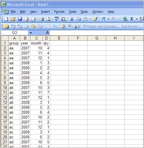
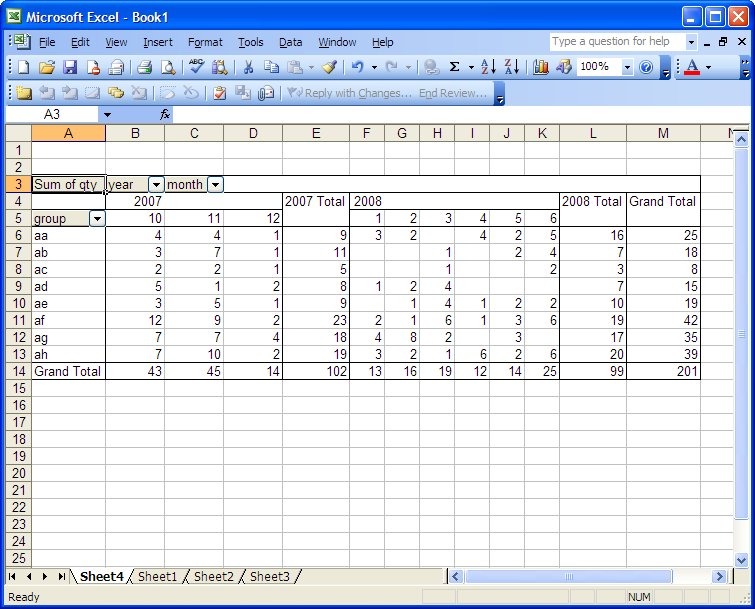
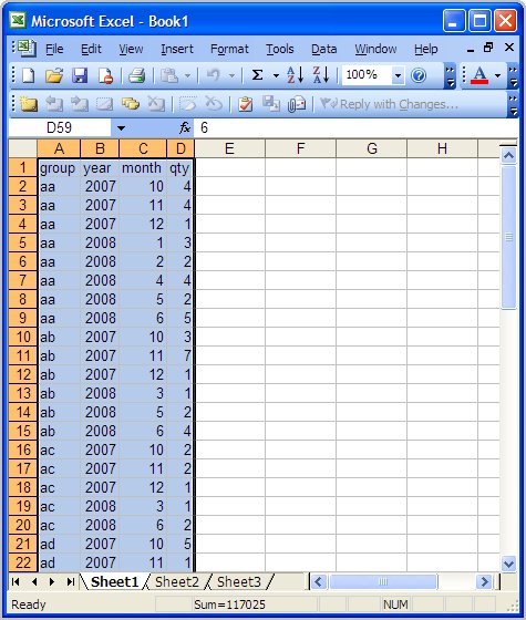
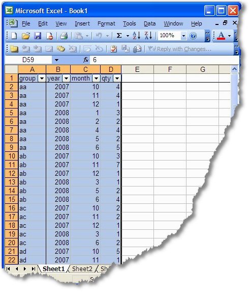
The goal is to take the information from the image on the right and pivot it to look like the table on the left.
After considerable searching, using keywords like rotate and transpose, I found nothing. After trial and error, I have found the way. The keyword is pivot.
Before pivoting the table, I wanted to use a filter to organize the existing table.
- Select all existing data
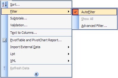
- From the toolbar, select Data > Filter > AutoFilter
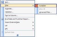
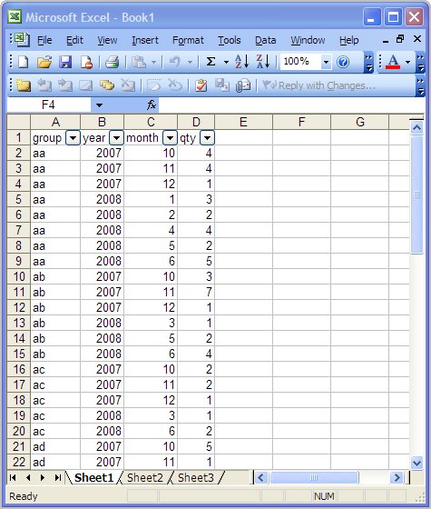
The result will look like the image below, notice now there are arrows at the top of each column. This permits the ability to filter the data to drill down to the desired results.
Next, I want to lock the window pane so that the top row will always be in view.
- Highlight one cell on the second row. Any cell, like A2, B2, C2, or D2.
- From the toolbar, select Windows > Freeze Panes
The result is the top row is now locked or frozen. Using the mouse to scroll through the data, row 1 will remain and note that the next row in this picture is 49.

Now that the existing data is more usable, the goal is to pivot the columns into rows.
- Select and highlight the columns.

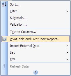
- From the toolbar, Data > PivotTable …..
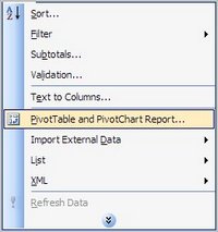
- This will launch the PivotTable and PivotChart Wizard
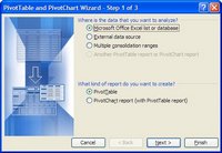
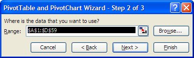
- Hit Next>
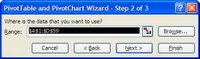
- Hit Next>

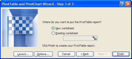
- Hit Finish

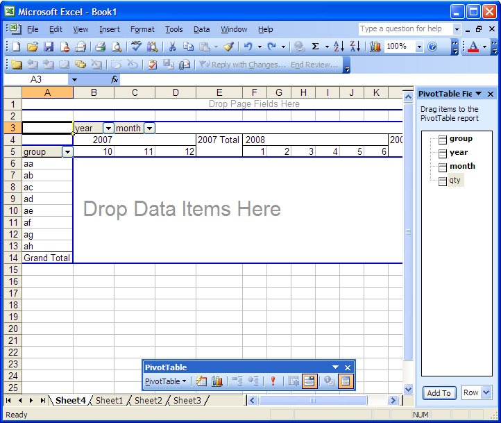
The result of the pivot table should look something like this.
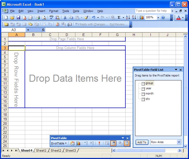
Drag from the PivotTable Field List to the desired location in the fields. In this case, I selected group and dragged to the far left.

Then, dragging the year then month, the table may look like this.
After dragging the qty over to the middle field, the result may look like this.
Note: The image below is an example without totals between rows. To remove or “hide” the totals between rows, simply select the row total cell in a row with a total, right click on it, and chose “hide”.

Done.